Phased Approach to Sediment Management
Phase 1:
Planning
Phase 2:
Developing a Sediment Budget
Phase 3:
Prioritizing Investments
The Planning Phase involved collecting data and identifying the relevant stakeholders – both users of the landscape as well as experts to get insights on the causes and impacts of sediment and erosion in the watershed.
In this phase, secondary research and existing data points on the issue of accelerated erosion/ sediment generation should be collated. Data should be used to:
Finalize the geographical scale and scope of the study (river basin, sub-river basin, catchment area, watershed)
Define the Socio-Economic characteristics and land use patterns of users within the landscape including putting together the best available Land use and Land Cover (LULC) maps
Identify the sources of the problem and collate all data available on these:
- Natural – topography, geology, rivers, rainfall, wind speeds etc
- Anthropogenic – grazing, deforestation, agriculture, road construction
- Temporal – Is the erosion seasonal, has it increased over the years?
- Spatial – Are there any hotspots of erosion, river catchments known for more erosion
List the key impacts of erosion and sedimentation
Identify current measures in place to tackle sediment generation/erosion
Identify institutions and stakeholder involved
Describe the policy framework (or lack of) to address the issue
Identify experts working on the issue
Understand the estimated amount of resources currently being used to address the problem
At this stage, it is also important to engage key partners and understand the extent and quality of data on sediment data available for the study area.
Engaging Key Partners
Sediment management at a basin or watershed scale is a complex issue involving several actors. There are various decision makers, knowledge, land holders and land users involved that all make up pieces in the sediment management puzzle. Undertaking a Stakeholder Analysis to understand the socio-economic dynamics and key actors interests and influence over processes of erosion and sedimentation is a key step at this stage.
Often in addressing sediment management there could be a key sector that actions are planned around. Two examples of sediment management executed through forging critical partnerships are highlighted below:
-
Key Partnerships for Sediment management in Kaligandaki Watershed, Nepal.
Nepal Electricity Authority (NEA), Department of Forests and Soil Conservation (DoFSC), Kathmandu University, Stanford University and World Bank.
The Kaligandaki A Hydropower Plant operated by the Nepal Electricity Authority (NEA) is Nepal’s largest power plant with an installed capacity of 144 MW and build at a cost of 350 million USD. Sediment management is required in the watershed to avoid huge losses that the plant faces due to sedimentation causing damage to equipment, loss of efficiency, loss of reservoir storage capacity and frequent repair and maintenance. To address the issue of sedimentation, the World Bank initiated a project to provide technical assistance and build capacities including on how changes in land management in the watershed could affect sediment delivery. Key partners in addressing sediment management were included the Department of Forests and Soil Conservation (DoFSC), Ministry of Forests and Environment, Government of Nepal, who have been investing in watershed management (referred to as “catchment area treatment”) activities for decades; the Gandaki Basin Management Centre which aims to provide a centralized knowledge platform for data, guidance, and best practices on watershed management in this region; The Natural Capital Project at Stanford University provided the technical leadership to undertake the Sediment modelling processes and Kathmandu University undertook field level data collection and analysis on sediment.
Key Partnerships for Sediment Management in the Upper Tana Watershed, Kenya.
Nairobi City Water & Sewerage Company (NCWSC) and Kenya Electricity Generating Company (KenGen), Tana and Athi River Development Authority (TARDA), The Nature Conservancy, ETC East Africa.
Nairobi in Kenya receives 95% of it’s water supply from the Tana River, originating in the highlands above Nairobi. Due to agricultural activities in these upper reaches, siltation of water has impacted downstream communities and reduced water supply and water quality to Nairobi. A few erosion and reservoir sedimentation studies to document the extent of sedimentation existed for the watershed. To address the challenge, the Upper Tana Nairobi Water Fund (UTNWF) was set up by The Nature Conservancy (TNC). To plan the fund, the economic impact of different land conservation interventions was modelled for three key basin stakeholders: small-holder farmers; Nairobi City Water & Sewerage Company (NCWSC) and Kenya Electricity Generating Company (KenGen). Land conservation measures further upstream in collaboration with small-holder farmers were deemed to hold mutual benefits - For example, reduced soil erosion was projected to increase agricultural yields and to increase water quality further downstream.
Sediment Data Availability
At this stage, stock of data and research on erosion and sediment in the basin should also be undertaken.
- Is data on sediment generation in the identified project area and key locations available?
- What are the data gaps and where does primary data need to be collected or supplemented?
- Determine time frame for collecting sufficient data
What is a Sediment Budget?
A Sediment budget is both an approach and a mathematical model. It is a rigorous quantitative accounting of the production, transfer and storage of sediment within a landscape. It identifies the magnitude of sediment sources and sinks in a watershed relative to watershed output. It provides a framework to organise and analyse information on sediment processes and their response to human interventions within a basin or watershed. It considers the processes of sediment generation as well as the sinks of sediment within an identified area.
- Processes identify the rates of sediment loss, the variables that determine sediment processes, the timing of generation and grain sizes and types of sediment.
- Sinks identify the rate of sediment that gets deposited on hill slopes and river channels or reservoirs.
Developing a Sediment Budget
The following section covers the process of how a sediment budget was prepared for the Kaligandaki Watershed in Nepal, which drains into the Kali Gandaki A Hydropower Plant.
Preparation of the Sediment Budget comprised of two key steps:
Step 1: Measuring the Quantity of the Sediment.
Step 2: Identifying the Sources of the Sediment.
Step 1: Measuring the Quantity of Sediment
Figure 1 Topography of the Watershed and location of gauging stations and their respective drainage area
Sediment Monitoring Campaign
The first step to understand where and how sediment is generated, sediment monitoring data at multiple locations throughout the watershed are needed. Incase such data sets are not available, a sediment monitoring campaign needs to be undertaken. Gauging stations to measure sediment delivery from sub-watersheds need to be installed and monitored over a period of one year. Suspended sediment samples should be collected weekly.
The sub-basin characteristics of where the gauging stations are installed should be captured including data on:
- Name of River or Tributary
- Description of Sub-basin (Upper, Mid, Lower, Plateau, Gorge etc)
- Drainage Area (Km2)
- Mean Elevation
- σ elevation [m]+
- Glaciation %
- Mean Annual Precipitation
Sediment Sampling and Load Calculations
The total suspended sediment discharge for each station can be calculated as
Q_S (t)=Q(t)*C_S (t)
With Q_S [t/d] and Q [m3/d] being the discharge of sediment and water, C_S being the sediment concentration [t/m3] and t denoting the day of the year when a sample was taken. To calculate the total annual load, assume that the load is constant between measurement dates.
Depending on the objective of monitoring sediment, values for bedload (gravels and coarser) can also be calculated.
Use of Sediment Rating Curves
Often there is better data available on discharge from monitoring stations than the sampling of sediment concentrations. This data can be used to extrapolate the sediment transport in past years without sediment observations by using sediment rating curves. This allows for a longer-term sediment budget and generalize results for a longer time period.
C_S=a*Q^b
where discharge is Q and sediment concentration 〖is C〗_S (a and b are regression parameters based on determining the optimal fit betwee the Q and Cs at monitoring stations)
Data Analysis
The Sample data from the Gauging Stations can provide data on sediment as Total Load (how much fine sediment is transported at the outlet of each sub-watershed in tonnes per year) year as well as Added Load (Indicates how much of that load originates within a sub-watershed)
The data highlights the relative contribution of sediment from each sub-basin. For instance, which basins contribute the most and the least sediment. The sub-basin characteristics such as rainfall combined with the data on sediment also reveal factors such as are the soils and hill-slopes hard to erode or is there high erosion?
Further, analyzing the mineral composition of the sediment can also yield information about the sediment generating process, and in the case of hydropower projects help assess their impacts on equipment. In Kaligandaki, Nepal, sediment composition was analyzed with regard to minerals Quartz, Feldspar and Tourmaline – all of which are harder than the chrome-nickel steel used for turbine parts.
Step 2: Identifying the Sources of the Sediment
Step 1 on sediment measurements from sub-watersheds gives an indication of the quantity of sediment being generated in sub-basins and which sub-basins may be contributing more and less sediment. What cannot be determined from the derived suspended load is which processes – eg. Deforestation, Landslides, roads or glaciers contributed to the sediment load. Thus, Step 2 of a Sediment Budget involves, understanding the contribution of these processes to the sediment load. The extent of erosion depends strongly on geographic setting, hydro-climatic conditions and human interference.
This is the stage where Sediment Models can be applied to identify the sources of sediment. Models can be used and adapted to measure the contribution of erosion from any or all the below:
Sheet, Rill and Gully Erosion
Glacial Erosion
Landslides and Rockfalls
Road Induced Erosion – Road Cuts
Road Induced Erosion – Road Surfaces
The most extensively developed and used Models are to measure Sheet and Gully Erosion (Water Erosion).
For the Kali Gandaki Watershed, the InVEST tool was used that applied the Revised Universal Soil Loss Equation (RUSLE) together with the Sediment Delivery Ratio.
Revised Universal Soil Loss Equation (RUSLE) enables the calculation of Average Soil Loss per unit of Area (plot area) using the formula:
A=R*K*LS*C*P
- A Erosion in t/ha/yr
- R is rainfall erosivity (units: MJ⋅mm/(ha⋅hr))
- K is soil erodibility (units: ton⋅ha⋅hr/(MJ⋅ha⋅mm)
- LS is a slope length-gradient factor (unitless)
- C is a cover management factor (unitless)
- P is a support practice factor
In the above equation, erosivity and erodibility are derived from gridded global data sets. The C values for different land use types (e.g., pasture vs. forests; derived from Nepal-specific land use maps) are derived from C values tabulated in relevant literature. The P factor can be used to parametrize the effectiveness of soil conservation practices to avoid soil runoff from a parcel (P=1: no effective erosion prevention, P=0: support practices fully stop soil runoff). A combination of C and P factors are used to describe the impact of a specific land use (e.g., growing corn) under different conservation practices (e.g., growing corn on a degraded, downslope-tilled plot vs. growing corn on a terraced plot with hedgerows).
The (RUSLE) calculates soil loss, not sediment yield, and the effects of erosion from other sources (such as gullies) and deposition within the field and broader landscape are not modelled.
Sediment Delivery Ratio
Eroded sediment will be transported downslope but a portion is deposited along the transport pathway. Retention of sediment on the slopes is modeled using a conceptual factor, commonly referred to as sediment delivery ratio (SDR), which is calculated for each pixel as a function of the area upslope of a pixel and the topography of the flow path between the pixel and the nearest stream (Cavalli et al., 2013). With the SDR applied, the final sediment delivery to the streams is
Q_(S,sheet)= E*SDR
The InVEST Sediment Delivery Ratio model works through the input of data into the model, and the output based on the data reflects as pixels or ‘cells’ simulating the outcomes of the data input.
| Sr No. | Input | Sources |
|---|---|---|
| 1. | Digital Elevation Model (DEM) | Satellite Images |
| 2. | Rainfall Erosivity Index (R Factor) | Global data sets, or rainfall data from rainfall gauging stations in study area |
| 3. | Soil Erodibility (K factor) | Global data sets, or Department of Irrigation/ Agriculture |
| 4. | Land Use Land Cover (LULC) | Best available LULC maps for the area/ secondary literature |
| 5. | Watersheds | Hydrology tool in the ArcMap |
| 6. | Biophysical Table (C and P factors) | Existing data (C and P factors) |
| 7. | Threshold Flow Accumulation | Global data sets |
View the rest of the Models used in the Kali Gandaki Sediment Budget here
Glacial Erosion
Run-off from the glacier, which mobilizes sediment at the glacier toe, the size of the glacier, and the properties of the underlying bed-rock, which typically results in a non-linear relationship between the sediment generation of a glacier and the produced melt water discharge Gangotri glacier in western Nepal Haritashya et al. (2006) propose a power law of the form
log(C_SS) = 1.0862 * log(Q_g) + 1.3141
where
- C_SS Suspended sediment concentration in g/m3
- Q_g Discharge from a glacier in m3/s
To determine discharge, we assume that the discharge can be determined from a steady state mass balance
▁(Q_g )=▁(P_g )-▁(ET_g )
Where
- ▁(Q_g ) mean discharge in m3/s
- ▁(P_g ) mean precipitation over a glacier in m3/s
- ▁(ET_g ) mean evapotranspiration from the glacier surface in m3/s
Landslides and Rockfalls
Often Landslides produce most of the sediment in watersheds in mountainous regions of South Asia. Given they are such an integral part of Watershed Projects, a dedicated guidance note on Landslide Risk Assessment note has been prepared
Road Induced Erosion – Road Cuts
Based on the width of a road, the local gradient of the hillslope into which the road is cut and making some assumptions on the cut slope angle. These parameters then allow to calculate the cross-section of the road cut on a specific slope, so that the total cut material from a specific road segment is
E_Cut^*=A_C L ρ_S
Where
- M_C^* Mass of cut material in t
- A_C cross sectional area of the road cut in m2
- L length of the road segment in m
- ρ_S sediment density in t/m3
Note that this equation yields the instantaneous sediment in tons mobilized when the road is cut (or when it needs to be cleared after a landslide). To calculate a rate of annual sediment delivery, the analysis assumed that sediment from the road cut is mobilized over a 25 year time horizon, so that the annual delivery is
E_Cut=(E_Cut^*)/25
Sediment delivery from the cut material to the stream is calculated using the pixel-specific SDR factor so that Q_(S, Cut)=E_Cut*SDR
Road Induced Erosion – Road Surfaces
Erosion from road surfaces is modelled for each road segment using an empirical equation
- E_R=(E_RS+E_CS )*ρ_S
- E_RS+E_CS=1.09*(-0.432+f_g (S^(1.5) P))*L*W
Variables are:
- E_R Total erosion from a road segment in t/yr
- E_RS Erosion from the road surface in t/yt
- E_CS Erosion from the cut slope in t/yr
- ρ_S Sediment density in t/m3
- f_g grading factor 4.73 for freshly graded roads, 1.88 for ungraded road. Average (3.305) was used for this study
- S gradient of road segment
- P precipitation in cm/yr
- L Length of road segment m
- W Width of road segment m
The analysis assumes that part of the sediment running off a road at its lowest point is retained on the landscape before reaching the stream. This retention is modelled using the same per-pixel SDR factor as used in the sheet erosion model (Box 3.1) so that the final sediment delivery to streams is
Q_(S,Roads)=E_R*SDRResults of a Sediment Budget
Sediment load from each sub-watershed to the streams (left) and the processes dominating sediment load in each sub-watershed in Kali Gandaki
-
Quantity of Sediment and Sources of Sediment mapped
The sediment measurements help determine the contribution of sediment in the watershed. The results of a sediment budget yield information on both quantity of sediment and sources of sediment. A comparison of observed sediment load and the multi-model approach can be used to verify the accuracy of the models.
Analysis of 2 Sediment Budgets
1. Sediment Budget of Kaligandaki Watershed:
As seen from the results of the Sediment Budget of the Kaligandaki watershed – landslides make up the largest part of the sediment budget for most watersheds followed by hill slope erosion (SDR – Sediment Delivery Ratio model). In comparison with these, glaciers are a contributing factor in high elevation sub-watersheds while roads are not dominant in any major sub-watershed.
Often there can be a great diversity in sediment load and yield within sub-watersheds, which is not necessarily aligned with the spatial distribution of rainfall. In the case of Kaligandaki watershed of Nepal, for instance, the tributary watersheds receiving most of the watershed’s precipitation did not contribute the most to its sediment budget.
Improved data of geologic factors such as lithology, uplift rates and fracturing of rocks along fault lines are critical for improving understanding of where and how sediment is generated in the watershed.
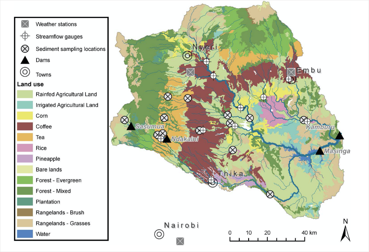
2. Sediment Budget of Upper Tana Watershed, Nairobi:
The results of the Sediment Budget of the Upper Tana Watershed reveal that natural areas in the higher mountain areas hardly contribute any sediment (3% of total basin sediment yield) while cultivated and grazed areas contribute most of the erosion and sediment. The main sediment producing areas are located on steep slopes. The main erosive areas identified were those where coffee is produced, with an average erosion rate of 50 t ha-1 year-1. The study also found that among the landuse rainfed category of rainfed agricultural land, plots where subsistence agriculture together with maize cultivation was undertaken erosion was a high average of 10 t ha-1 year-1
QUANTITY
SOURCE
Prioritizing Interventions based on findings
One of the principle outcomes of evidence based research and targeted studies on sediment modelling is to be able to determine the priority sites and key interventions that can address the challenges posed by accelerated erosion and sediment. As mentioned at the start of the guidance note – while the end objective maybe to improve agricultural productivity, hydropower efficiency, or quality of drinking water supplies – the findings can yield important findings on
- Priority sites generating the maximum erosion and sediment
- Locations where maximum benefits from watershed management can be achieved (This maybe different from sites generating the most sediment as it may not be possible in all instances to stop the erosion, for instance glacial sedimentation).
- Types of interventions such as afforestation, check dams, change in agriculture practices, and other ‘green infrastructure’ measures known to reduce erosion.
The processes and levels of specificity for prioritizing interventions have become increasingly more accurate and sophisticated with the application of sediment modelling processes and economic models involving cost-benefit analysis.
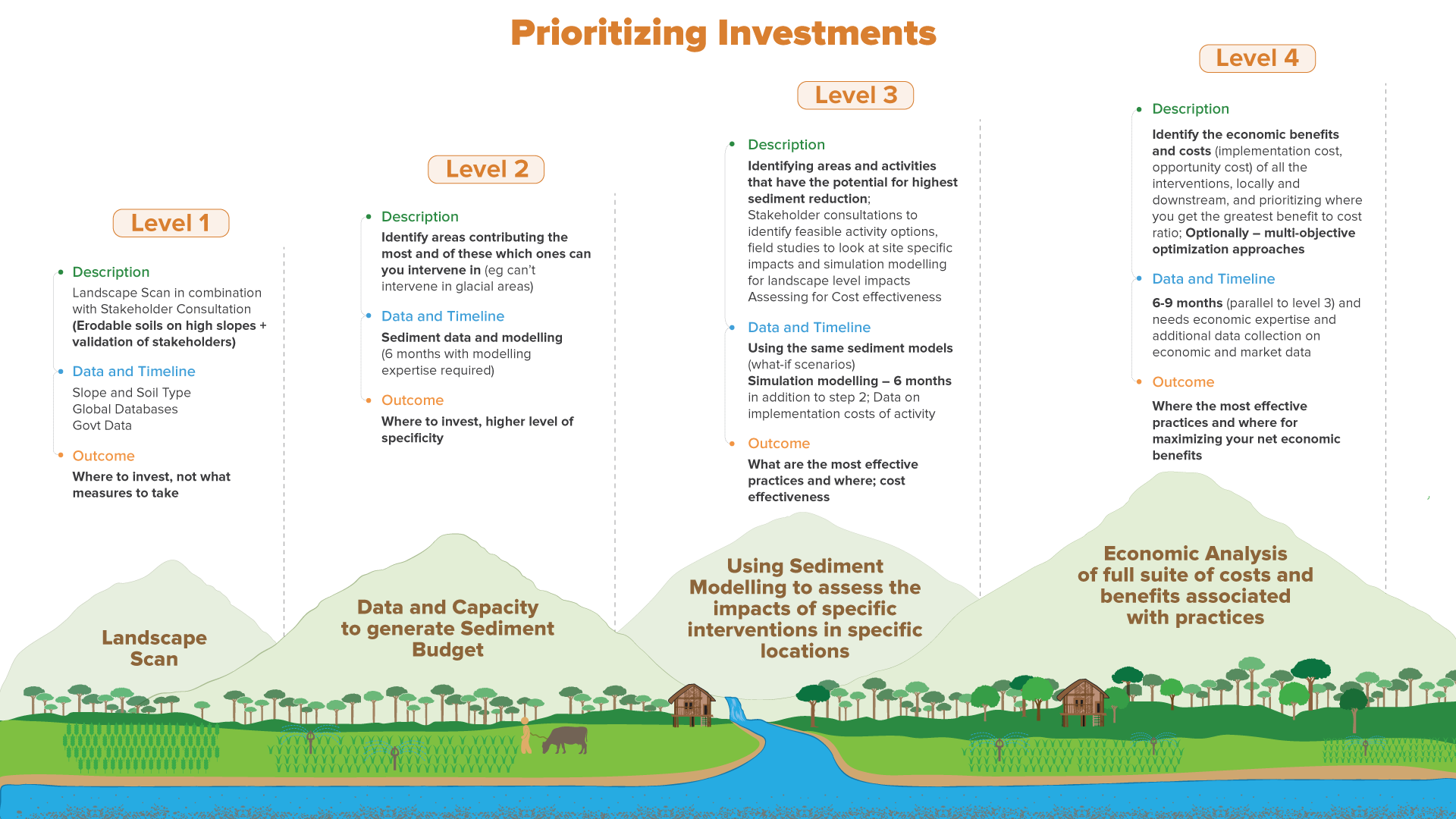
However, even without the use of full suite of modelling and cost-benefit tools, the prioritization process is highly beneficial and can be undertaken at different levels based on data availability and budgetary considerations. This chapter outlines four different levels ranging from basic to more advanced levels of specificity that can be achieved to determine how to prioritize where to intervene in the watershed and what interventions might work best.
Level 1: Landscape Scan and Stakeholder Consultations
Level 2: Preparation of Sediment Budget and Identification of Priority Sites
Level 3: Sediment Modelling to assess impacts of specific interventions in targeted locations
Level 4: Economic Analysis of full suite of costs and benefits associated with practices
Level 1: Landscape Scan and Stakeholder Consultations
| Description | Data & Timeline | Output & Outcome |
|---|---|---|
| The Landscape Scan is useful for understanding the current scenario of erosion using qualitative and quantitative data; It is the most basic level of prioritization that can be undertaken with basic data – such as known locations of erodible soils and validation through stakeholder consultations. It may not be beneficial to understand historic trends or changes related to sediment in the landscape, or to define the efficacy of specific interventions. | Slope and Soil Type Global Databases Government Data (Line departments such as forest department, agriculture department, Irrigation department) Time: 1 – 5 months. | Where to invest (not enough to define what measures to take). |
Level 2: Preparation of Sediment Budget and Identification of Priority Sites
| Description | Data & Timeline | Output & Outcome |
|---|---|---|
| Using a sediment budget, one can Identify areas contributing the most sediment as well as those where interventions cannot take place (eg can’t intervene in glacial areas) and prioritize where to invest. | Data: Sediment data and results of modelling (quantity and source) Time: 6 months with modelling expertise required. |
Where to invest, higher level of specificity. |
Level 3: Sediment Modelling to assess impacts of specific interventions in targeted locations
| Description | Data & Timeline | Output & Outcome |
|---|---|---|
| Sediment models can also be used to identify areas and activities that have the potential for highest sediment reduction; This can be combined with stakeholder consultations to identify feasible activity options, field studies to look at site specific impacts and simulation modelling for landscape level impacts. At this level an exercise to understand cost effectiveness based on activities identified can be undertaken by using government data and through stakeholder consultations to understand the cost/hectare of specific interventions. | Using the same sediment models (what-if scenarios) Simulation modelling – 6 months in addition to step 2; Data on implementation costs of activity. | What are the most effective practices and locations they should be implemented in; cost effectiveness of activities. |
Level 4: Economic Analysis of full suite of costs and benefits associated with practices
| Description | Data & Timeline | Output & Outcome |
|---|---|---|
| Identify the economic benefits and costs (implementation cost, opportunity cost) of all the interventions, locally and downstream, and prioritizing where you get the greatest benefit to cost ratio; Using this method, the net present value (NPV) of benefit streams from watershed management activities is calculated. These could include dollar values calculated for i) reduction in sediment benefiting hydropower projects, ii) avoided damages to structures and roads due to landslide mitigation, iii) changes in carbon stocks and iv) on-site benefits to landholders. A cost benefit analysis can be used to determine the economic value for an optimum investment portfolio. For example, in Kaligandaki study it was established that with a budget of US$ 500,000 each dollar invested in watershed management yields $4.38 in benefits. At this level, one can also undertake a multi-objective optimization approach such as a ROOT analysis. ROOT calculates optimal portfolios of restoration locations to support multiple ecosystem service objectives. |
6-9 months (parallel to level 3) and needs economic expertise and additional data collection on economic and market data. | Locations for the most effective practices and locations for maximizing your net economic benefits. |